The GAIA-DEM data archive provides to the solar community Quick look AIA/SDO DEM maps at a 30-min cadence. The corresponding FITS files can be downloaded starting from 2010/05/13.

1.1 Purpose

The purpose of the Gaussian AIA DEm Maps (GAIA-DEM) database is to provide on one hand, synoptic Gaussian DEM inversions of the AIA data, and on the other hand, new tools to facilitate the interpretation, using the results of Guennou et al. 2012a and Guennou et al. 2012b (hereafter respectively Paper I and Paper II). The AIA instrument (Atmospheric Imaging Assembly; Lemen et al. 2012) on board SDO (Solar Dynamics Observatory: Pesnell et al., 2011) is a set of normal incidence imaging telescopes, observing the Sun at high spatial resolution (0.6 pixels) and high cadence (typically 12 s). Six coronal bands are available: 94, 131, 171, 193, 211, and 335 Å. Compared to previous instruments, the multiplication of pass-bands provides new possibilities to reliably estimate the DEM simultaneously over a large FOV.

48 inversions per day at a 30-min cadence are generally available to download. The SDO DEM inversion pipeline provides the best fit matching the observations, assuming that the DEM is a Gaussian (in logarithmic scale). Four map of parameters, corresponding to the parametrization of the DEM, are provided: the total Emission Measure (EM), the central temperature T_c, the thermal width σ (corresponding to the width of the Gaussian) and the residual χ² giving information about the pertinence of the model.

1.2 Background

The differential Emission Measure (or DEM) is one of the most used diagnostic tools for solar and stellar plasmas, defined as follow



The DEM provides a measure of the amount of emitting plasma as a function of temperature. As defined by Craig & Brown (1976), n_e² is the mean square electron density over the regions dp of the Line-Of-Sight (LOS) at temperature T_e, weighted by the inverse of the temperature gradients in these regions. Given a set of observations in N different bands, the DEM can in principle be inferred by reversing the signal acquisition process described by the following equation (Pottasch, 1964)
where R_b is the temperature response function of a given instrument in a spectral band b. Solving the DEM integral equation implies reversing the image acquisition, LOS integration, and photon emission processes to derive the distribution of temperature in the solar corona from observed spectral line intensities. However, to solve for the DEM is a very challenging task, partly due to the technical issues, but also due to the intrinsic underconstraint of inverse problems and to the inevitable presence of random and systematic errors. The intrinsic difficulties involved in this inverse problem lead to many complications in its inference, making its interpretation ambiguous. Despite these difficulties, the DEM diagnostic tool has been extensively used in the past several decades, for most types of coronal structures.
In this perspective, we recently developed a technique to provide new tools for systematically and completely characterize the DEM inversion, and assisting the DEM interpretation (see Papers I and II). This method, based on Monte-Carlo simulations of the random and systematic errors, is able to systematically explore the whole space of solutions, in order to determine their respective probabilities and to quantify the robustness of the inversion. Using a Gaussian description of the DEM to limit the number of parameters, while still represents a variety of plasma conditions (from isothermal to greatly multithermal, varying the Gaussian width), the inversion technique provides the best fit through a least-square inversion comparing the observations with the theoretical expectations.

2.1 Why Gaussian DEMs?

There is no fundamental reason for the solar plasma to have a Gaussian DEM. However, Gaussians are a good first order approximation to determine the main characteristics of the DEM. The degree of multithermality of the plasma can be assessed, through the parameter σ (width of the Gaussian). The central temperature T_c gives indications of the mean plasma temperature along the LOS. Furthermore it has the advantage to be a simple parameterization and this allows the detection of secondary solutions and the computation of their respective probabilities (more on this below). Section 3 gives guidelines to properly interpret the results. In particular, the interpretation of the χ² values is discussed.
2.2 Data processing
To improve the signal to noise ratio in some bands, in particular in the 94 and 335Å channels, the data are temporally and spatially summed. First, the data in all channels are co-registered, and then, 10 consecutive images are summed (one image per minute) for each channel. Final image in each channel is then obtained by spatially binning the images by a factor 4 (4096x4096 → 1024x1024).

2.3 Minimization

The inverted DEM ξ^I is evaluated by least-squares minimization of the distance between the theoretical intensities and the AIA observations, through the following criterion C(ξ)

where b is one of the AIA channels, ξ is a DEM model (Gaussian in this case) and a_b^u is obtained by summing quadratically the standard deviations of the four individual contributions to the uncertainties: photon noise, read noise, calibration, and atomic physics (see Paper I for more details about the estimation of the uncertainties). The temperature response functions, necessary to compute the theoretical intensities, have been estimated using Chianti 7.1 (Dere et al. 2009) and the function aia_get_response of the SSW package (see Boerner et al, 2012). Then, the I_b^th have been computed assuming a Gaussian DEM model defined as



   Fig. 1: Different Gaussian DEMs, obtained for different thermal widths, from 0.01 to 0.6, but with the same total Emission Measure of 10²⁸cm^-5.
Constraining the solutions to be Gaussian has additional advantages. Indeed, if the DEM is fully determined by a limited number of parameters, one can regularly sample the parameter space and compute once and for all the corresponding theoretical intensities I_b^th. The theoretical expectations have been computed using CHIANTI from log(T_e) = 5 to log(T_e) = 7.5 in steps of 0.005 log(T_e). The EM varies over a wide range from 10²⁵ cm^-5to 10³³ cm^-5 in steps of 0.04 log(EM) and the DEM width varies linearly in 80 steps from σ = 0 to σ = 0.8 log(Te). These parameters are reminded in the fits files headers, through the keywords TMIN, TMAX and DSIGMA. Therefore, this choice of sampling leads to easily manageable criterion cubes (one per wavelength) and then, the inverted DEM is given by the set of parameters EM^I, T_c^I and σ^I minimizing the criterion C(ξ).

3.1 General View

The technique presented in Paper I and Paper II is a useful tool to assist the DEM interpretation, by providing a complete statistical characterization of the DEM inversion. The probability maps presented in this work (in particular in Paper II, section 3), computed via Monte-Carlo simulations, and taking into account the random and systematic errors, provide important information about the reliability of the results. Such maps, providing the conditional probability that the plasma has a given DEM ξ^P knowing the results of the inversion ξ^I, provide all possible Gaussian DEMs, and their associated probabilities, which are consistent with the inversion results. Secondary solutions, if any, possibly leading to an erroneous conclusion regarding the thermal structure of the solar corona, can be thus identified, and their probabilities can be quantified.



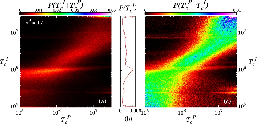
  Fig. 2: Probability maps for the central temperature parameter of the DEM, obtained using our simulations developed in Paper I and II. The left panel gives the probability to obtain a given solution knowing the input. The right panel can be used to interpret the inversion results, reading horizontally the probability distributions (see Paper II, section 3.2 for more details)

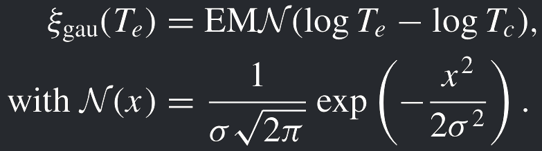
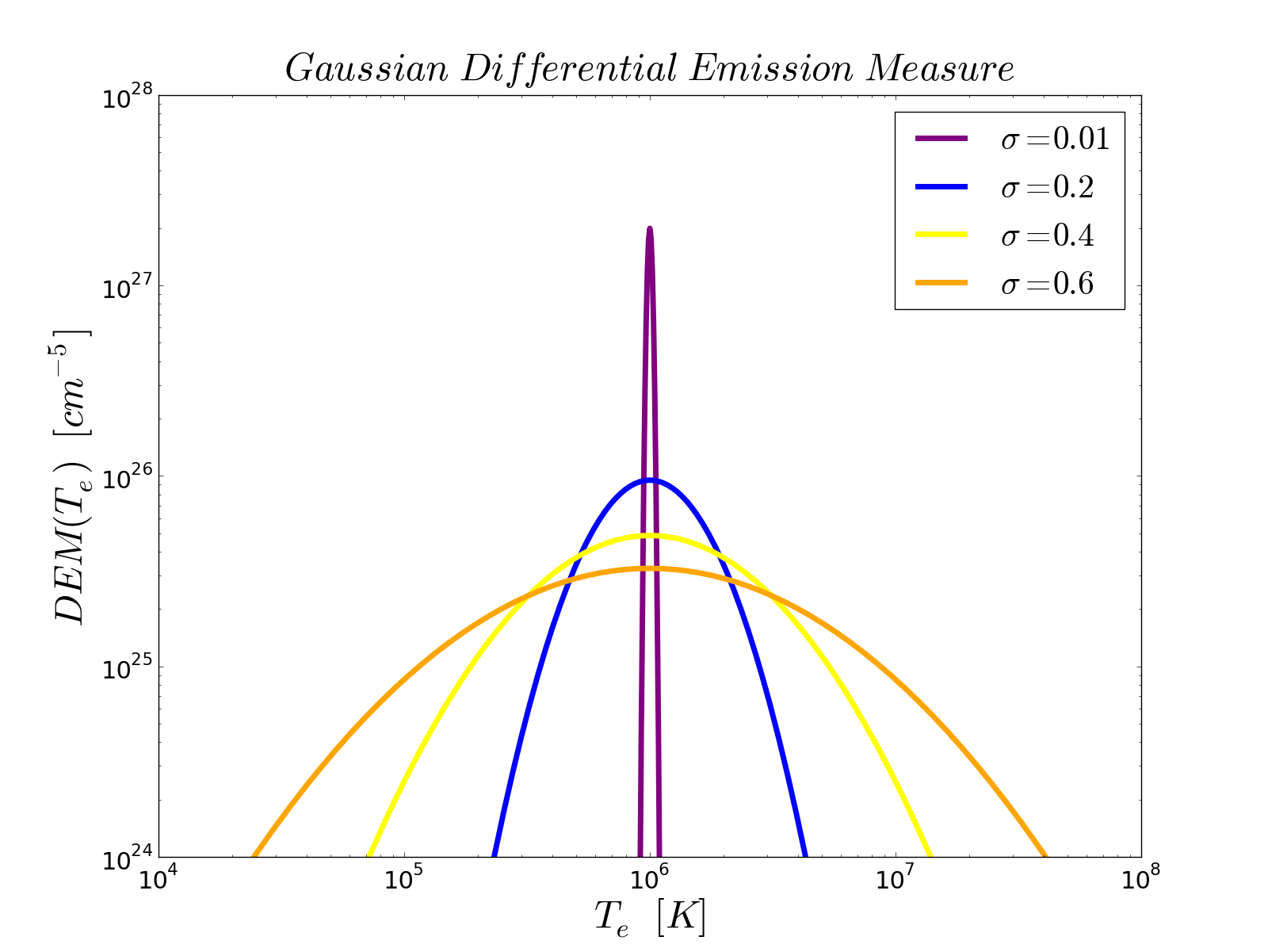
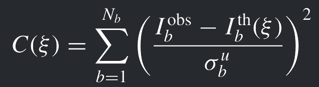
The Gaussian DEM model can be realistic for polar coronal holes (see Hahn et al, 2011), but it can also be inappropriate for other structures. Indeed, studies of active regions show that the coolwards wing of their DEM generally follows a power law T^α where α is the slope of the DEM in a log-log scale (see Warren et al. 2011; Winebarger et al. 2011; Tripathi et al. 2011; Warren et al. 2012). In the case of active region, the interpretation of the Gaussian DEM can be more difficult, because the Gaussian is likely not to be a representative model of reality. But the analysis of the residuals χ² can guide the interpretation, considering that a great χ² corresponds to a poor adequacy between the model used to perform the inversion and the “real” DEM. The numerical experiments of Paper I and II have shown that if the plasma is truly Gaussian, 50% of the χ² values are between 0 and 4. When inverting real data, (the true DEM having no reason to be Gaussian), if the χ² is smaller than 4 we conclude that a Gaussian model is consistent with the data because we would have 50% chance to obtain the same result if the plasma was truly Gaussian.

3.2 How to understand the on-line plots?

A preview of each DEM parameter and of the residuals is available on-line, as follow:



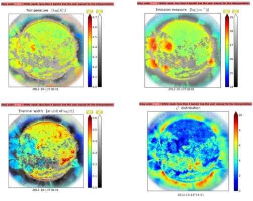
On the Temperature, Emission Measure and Thermal Width plots, two different colorbars are given:

      1. one colorbar (from blue to red) corresponding to the pixels where the values of the χ² < 4. The Gaussian DEM model, used to compute the theoretical intensities can be considered in good agreement with the observations.
      2. The second colorbar (in a gray scale), corresponding to the pixels where χ² > 4. In this case, the Gaussian DEM model can be considered inconsistent with the observations (or at least less likely not to be a good model).


The two scales allow the user to quickly determine the reliable areas in the DEM parameter maps. A message is present on the four parameter maps, reminding the user to be careful with the interpretation. The date, written below the main panel on each parameter map, corresponds to the mean date of the observations used (see Section 2-a of this user manual for more details).

The white mask present on each image corresponds to the pixels where the signal is > 1 DN in, at least, one of the six bands. Considering the difficulties highlighted in Paper I and II in the DEM robustness, we choose to perform the DEM inversion only where all the six bands present a significant response.

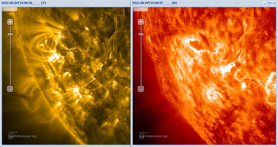
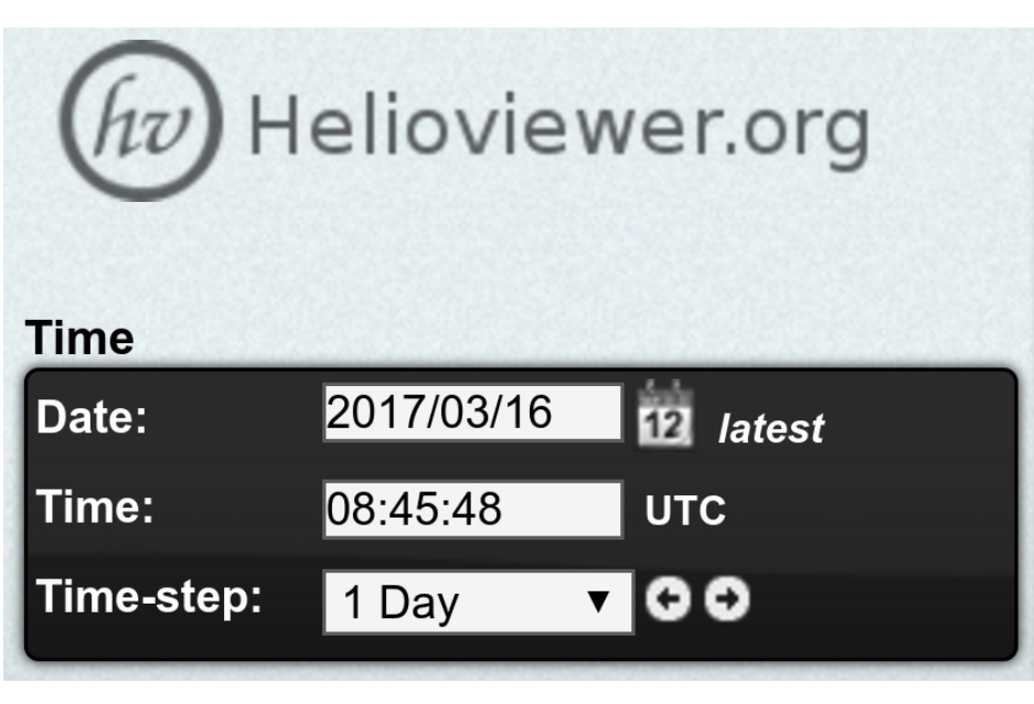
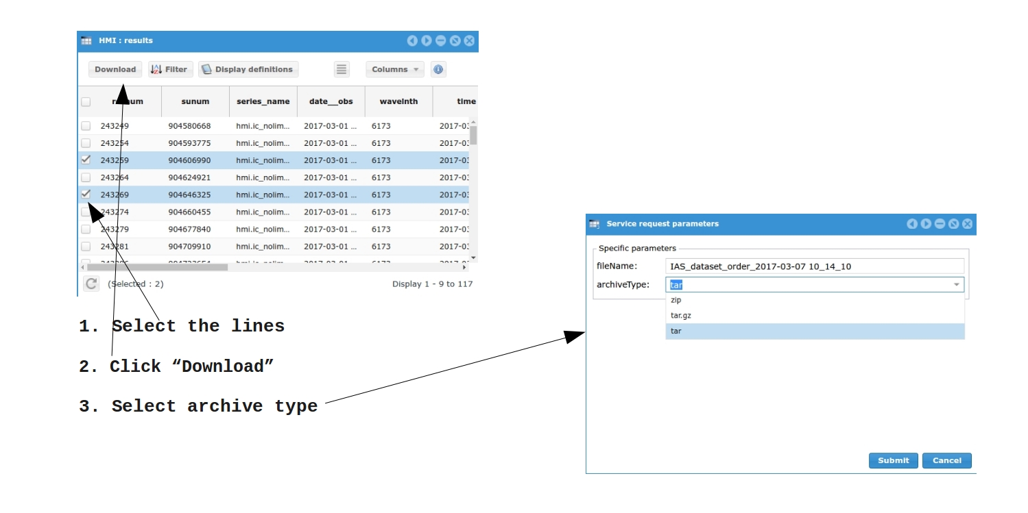
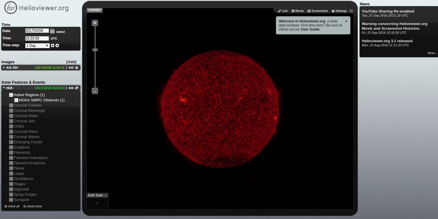
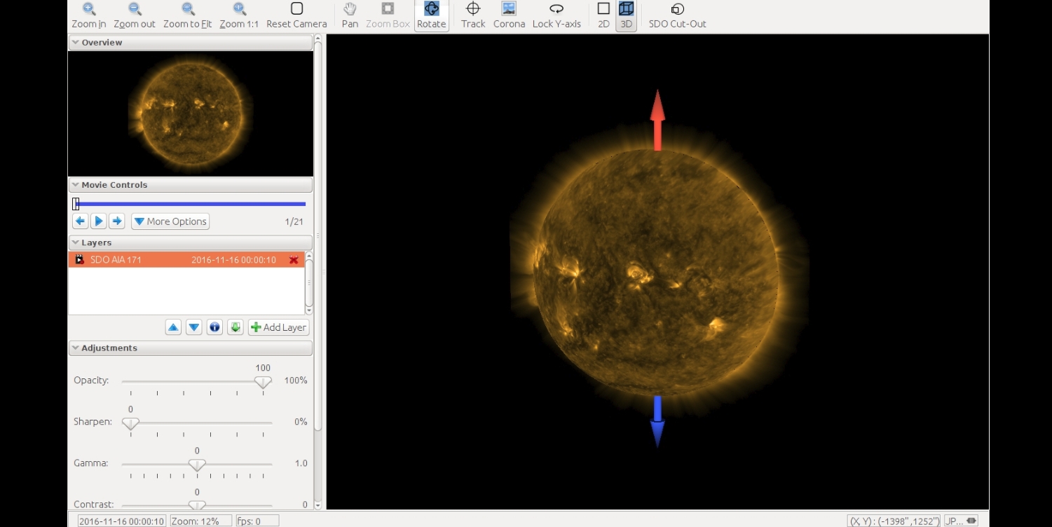
In addition, it can be interesting to display the initial SDO/AIA preview images. This can be done by using the links preview in the Helioviewer column. By clicking on any of these links, you first obtain the link for all the six coronal channel instrument, and then, the browser will open the Helioviewer interface and show the AIA image corresponding to the wavelength you've clicked on. The corresponding date will be the mean date (or the closest date available with helioviewer.org) of the observations used. Usual GoogleEarth-like mouse functions are available to zoom and pan in the image.

Before downloading the data corresponding to your query, it can be interesting to display a few preview images. This can be done by using the links preview in the Helioviewer column. By clicking on any of these links, the browser will open a window with the Hhelioviewer.org interface (using its instance at MEDOC/IAS) and show the AIA image corresponding to the wavelength and date you' have clicked on (or the closest date available ).

In this window, the mouse can be used to zoom and pan in the image.

This paragraph is intended for the users that have already downloaded some data from this site and that need help to read the FITS files. The paragraph just gives some hints about how to use the AIA level 1 files, but the user should refer to JSOC's documentation(http://www.lmsal.com/sdodocs/) for a complete description of how to analyze the AIA data.

2.1 How to visualize Rice-compressed FITS files

First untar (or unzip) the downloaded archive file.
Each item contained in this archive is a FITS file compressed with Rice-compression. To read an image in IDL, you can use the following line of code :
       image = readfits( fits_filename_after_untar, EXTEN=1, /FPACK )
This line of IDL code uses the /FPACK keyword that calls the external funpack executable provided by NASA's FITSIO's FPACK library
To display on screen the 4096x4096 image that is now loaded, you can use the following :
      tvscl, alog( rebin(image,1024,1024)>0.1 )

2.2 How to visualize decompressed FITS files with IDL

In IDL, just read the FITS file using the readfits function :
Each item contained in this archive is a FITS file compressed with Rice-compression. To read an image in IDL, you can use the following line of code :
       image = readfits( downloaded_fits_filename )
To display on screen the 4096x4096 image that is now loaded, you can use the following :
      tvscl, alog( rebin(image,1024,1024)>0.1 )